Training a Variational Auto-Encoder
This guide will give a quick guide on training a variational auto-encoder (VAE) in torchbearer. We will use the VAE example from the pytorch examples here:
Defining the Model
We shall first copy the VAE example model.
class VAE(nn.Module):
    def __init__(self):
        super(VAE, self).__init__()

        self.fc1 = nn.Linear(784, 400)
        self.fc21 = nn.Linear(400, 20)
        self.fc22 = nn.Linear(400, 20)
        self.fc3 = nn.Linear(20, 400)
        self.fc4 = nn.Linear(400, 784)

    def encode(self, x):
        h1 = F.relu(self.fc1(x))
        return self.fc21(h1), self.fc22(h1)

    def reparameterize(self, mu, logvar):
        if self.training:
            std = torch.exp(0.5*logvar)
            eps = torch.randn_like(std)
            return eps.mul(std).add_(mu)
        else:
            return mu

    def decode(self, z):
        h3 = F.relu(self.fc3(z))
        return torch.sigmoid(self.fc4(h3))

    def forward(self, x):
        mu, logvar = self.encode(x.view(-1, 784))
        z = self.reparameterize(mu, logvar)
        return self.decode(z), mu, logvar
Defining the Data
We get the MNIST dataset from torchvision, split it into a train and validation set and transform them to torch tensors.
BATCH_SIZE = 128

transform = transforms.Compose([transforms.ToTensor()])

# Define standard classification mnist dataset with random validation set

dataset = torchvision.datasets.MNIST('./data/mnist', train=True, download=True, transform=transform)
splitter = DatasetValidationSplitter(len(dataset), 0.1)
basetrainset = splitter.get_train_dataset(dataset)
basevalset = splitter.get_val_dataset(dataset)
The output label from this dataset is the classification label, since we are doing a auto-encoding problem, we wish the label to be the original image. To fix this we create a wrapper class which replaces the classification label with the image.
class AutoEncoderMNIST(Dataset):
    def __init__(self, mnist_dataset):
        super().__init__()
        self.mnist_dataset = mnist_dataset

    def __getitem__(self, index):
        character, label = self.mnist_dataset.__getitem__(index)
        return character, character

    def __len__(self):
        return len(self.mnist_dataset)
We then wrap the original datasets and create training and testing data generators in the standard pytorch way.
trainset = AutoEncoderMNIST(basetrainset)

valset = AutoEncoderMNIST(basevalset)

traingen = torch.utils.data.DataLoader(trainset, batch_size=BATCH_SIZE, shuffle=True, num_workers=8)

valgen = torch.utils.data.DataLoader(valset, batch_size=BATCH_SIZE, shuffle=True, num_workers=8)
Defining the Loss
Now we have the model and data, we will need a loss function to optimize. VAEs typically take the sum of a reconstruction loss and a KL-divergence loss to form the final loss value.
def binary_cross_entropy(y_pred, y_true):
    BCE = F.binary_cross_entropy(y_pred, y_true, reduction='sum')
    return BCE
def kld(mu, logvar):
    KLD = -0.5 * torch.sum(1 + logvar - mu.pow(2) - logvar.exp())
    return KLD
There are two ways this can be done in torchbearer - one is very similar to the PyTorch example method and the other utilises the torchbearer state.
PyTorch method
The loss function slightly modified from the PyTorch example is:
def loss_function(y_pred, y_true):
    recon_x, mu, logvar = y_pred
    x = y_true

    BCE = bce_loss(recon_x, x)

    KLD = kld_Loss(mu, logvar)

    return BCE + KLD
This requires the packing of the reconstruction, mean and log-variance into the model output and unpacking it for the loss function to use.
    def forward(self, x):
        mu, logvar = self.encode(x.view(-1, 784))
        z = self.reparameterize(mu, logvar)
        return self.decode(z), mu, logvar
Using Torchbearer State
Instead of having to pack and unpack the mean and variance in the forward pass, in torchbearer there is a persistent state dictionary which can be used to conveniently hold such intermediate tensors. We can (and should) generate unique state keys for interacting with state:
# State keys
MU, LOGVAR = torchbearer.state_key('mu'), torchbearer.state_key('logvar')
By default the model forward pass does not have access to the state dictionary, but torchbearer will infer the state argument from the model forward.
from torchbearer import Trial

torchbearer_trial = Trial(model, optimizer, loss, metrics=['acc', 'loss'],
                          callbacks=[add_kld_loss_callback, save_reconstruction_callback()]).to('cuda')
We can then modify the model forward pass to store the mean and log-variance under suitable keys.
    def forward(self, x, state):
        mu, logvar = self.encode(x.view(-1, 784))
        z = self.reparameterize(mu, logvar)
        state[MU] = mu
        state[LOGVAR] = logvar
        return self.decode(z)
The reconstruction loss is a standard loss taking network output and the true label
loss = binary_cross_entropy
Since loss functions cannot access state, we utilise a simple callback to combine the kld loss which does not act on network output or true label.
@torchbearer.callbacks.add_to_loss
def add_kld_loss_callback(state):
    KLD = kld(state[MU], state[LOGVAR])
    return KLD
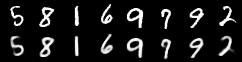
Visualising Results
For auto-encoding problems it is often useful to visualise the reconstructions. We can do this in torchbearer by using another simple callback. We stack the first 8 images from the first validation batch and pass them to torchvisions save_image function which saves out visualisations.
def save_reconstruction_callback(num_images=8, folder='results/'):
    import os
    os.makedirs(os.path.dirname(folder), exist_ok=True)

    @torchbearer.callbacks.on_step_validation
    def saver(state):
        if state[torchbearer.BATCH] == 0:
            data = state[torchbearer.X]
            recon_batch = state[torchbearer.Y_PRED]
            comparison = torch.cat([data[:num_images],
                                    recon_batch.view(128, 1, 28, 28)[:num_images]])
            save_image(comparison.cpu(),
                       str(folder) + 'reconstruction_' + str(state[torchbearer.EPOCH]) + '.png', nrow=num_images)
    return saver
Training the Model
We train the model by creating a torchmodel and a torchbearertrialand calling run. As our loss is named binary_cross_entropy, we can use the ‘acc’ metric to get a binary accuracy.
model = VAE()
optimizer = optim.Adam(filter(lambda p: p.requires_grad, model.parameters()), lr=0.001)
loss = binary_cross_entropy

from torchbearer import Trial

torchbearer_trial = Trial(model, optimizer, loss, metrics=['acc', 'loss'],
                          callbacks=[add_kld_loss_callback, save_reconstruction_callback()]).to('cuda')
torchbearer_trial.with_generators(train_generator=traingen, val_generator=valgen)
torchbearer_trial.run(epochs=10)
This gives the following output:
0/10(t): 100%|██████████| 422/422 [00:01<00:00, 219.71it/s, binary_acc=0.9139, loss=2.139e+4, running_binary_acc=0.9416, running_loss=1.685e+4]
0/10(v): 100%|██████████| 47/47 [00:00<00:00, 269.77it/s, val_binary_acc=0.9505, val_loss=1.558e+4]
1/10(t): 100%|██████████| 422/422 [00:01<00:00, 219.80it/s, binary_acc=0.9492, loss=1.573e+4, running_binary_acc=0.9531, running_loss=1.52e+4]
1/10(v): 100%|██████████| 47/47 [00:00<00:00, 300.54it/s, val_binary_acc=0.9614, val_loss=1.399e+4]
2/10(t): 100%|██████████| 422/422 [00:01<00:00, 232.41it/s, binary_acc=0.9558, loss=1.476e+4, running_binary_acc=0.9571, running_loss=1.457e+4]
2/10(v): 100%|██████████| 47/47 [00:00<00:00, 296.49it/s, val_binary_acc=0.9652, val_loss=1.336e+4]
3/10(t): 100%|██████████| 422/422 [00:01<00:00, 213.10it/s, binary_acc=0.9585, loss=1.437e+4, running_binary_acc=0.9595, running_loss=1.423e+4]
3/10(v): 100%|██████████| 47/47 [00:00<00:00, 313.42it/s, val_binary_acc=0.9672, val_loss=1.304e+4]
4/10(t): 100%|██████████| 422/422 [00:01<00:00, 213.43it/s, binary_acc=0.9601, loss=1.413e+4, running_binary_acc=0.9605, running_loss=1.409e+4]
4/10(v): 100%|██████████| 47/47 [00:00<00:00, 242.23it/s, val_binary_acc=0.9683, val_loss=1.282e+4]
5/10(t): 100%|██████████| 422/422 [00:01<00:00, 220.94it/s, binary_acc=0.9611, loss=1.398e+4, running_binary_acc=0.9614, running_loss=1.397e+4]
5/10(v): 100%|██████████| 47/47 [00:00<00:00, 316.69it/s, val_binary_acc=0.9689, val_loss=1.281e+4]
6/10(t): 100%|██████████| 422/422 [00:01<00:00, 230.53it/s, binary_acc=0.9619, loss=1.385e+4, running_binary_acc=0.9621, running_loss=1.38e+4]
6/10(v): 100%|██████████| 47/47 [00:00<00:00, 241.06it/s, val_binary_acc=0.9695, val_loss=1.275e+4]
7/10(t): 100%|██████████| 422/422 [00:01<00:00, 227.49it/s, binary_acc=0.9624, loss=1.377e+4, running_binary_acc=0.9624, running_loss=1.381e+4]
7/10(v): 100%|██████████| 47/47 [00:00<00:00, 237.75it/s, val_binary_acc=0.97, val_loss=1.258e+4]
8/10(t): 100%|██████████| 422/422 [00:01<00:00, 220.68it/s, binary_acc=0.9629, loss=1.37e+4, running_binary_acc=0.9629, running_loss=1.369e+4]
8/10(v): 100%|██████████| 47/47 [00:00<00:00, 301.59it/s, val_binary_acc=0.9704, val_loss=1.255e+4]
9/10(t): 100%|██████████| 422/422 [00:01<00:00, 215.23it/s, binary_acc=0.9633, loss=1.364e+4, running_binary_acc=0.9633, running_loss=1.366e+4]
9/10(v): 100%|██████████| 47/47 [00:00<00:00, 309.51it/s, val_binary_acc=0.9707, val_loss=1.25e+4]
The visualised results after ten epochs then look like this: